Decentralized computing systems like blockchains, oracles, and prover markets require incentives to be set appropriately in order for the system to operate at optimal efficiency. In these systems, there are users who have demand for compute requests (e.g. transactions, proofs, API requests, etc.), and there are nodes (e.g. validators, provers, oracles) who supply computation. Implicit in the design of a decentralized computing system is a protocol that (i) determines which user requests get service and which nodes provide service, and (ii) given that allocation of user requests to nodes, determines how much users pay for service, and how much nodes receive as payment for service.

Both decisions about the allocation of requests to nodes and pricing/payment must be made in the presence of many constraints, and these constraints make it very challenging to design systems that are optimally efficient. For example, only some allocations of user requests to nodes may be valid: nodes have compute limits and a given request may require a diverse collection of node resources. A request may even require the resources of multiple nodes (this is true e.g. in a blockchain, where transactions must be redundantly executed by many validators). An efficient allocation of requests to nodes not only satisfies all of those constraints, but also maximizes the economic value generated by the allocation by providing service to requests who are willing to pay the most and utilizing the nodes who can do the work at the lowest cost. And when it comes to pricing and payment, the protocol must choose payments that are low enough that users will accept them while providing rewards to nodes that are high enough that they’ll choose to provide service.

Designers of decentralized computing systems therefore have to manage a delicate balance between tractability and efficiency. If the system is very expressive and allows users and nodes to specify more complex constraints, then it may become intractable to find feasible allocations of requests to nodes that satisfy those constraints. The protocol also needs information about how much users are willing to pay and how much nodes pay in costs in order to find an efficient allocation and pricing/payment. Acquiring this information is difficult: direct elicitation in the form of bidding may fail or lead to distorted results due to the strategic behavior of users and nodes, preventing the protocol from efficiently utilizing its scarce resources. Furthermore, the hassle of bidding may in its own right deter users from using the system. For example, notice that even though most blockchains (e.g. Bitcoin, Ethereum, Solana) allocate resources at the protocol level by eliciting bids for transaction inclusion, most users prefer to use a wallet that bids on their behalf instead of placing bids themselves. Thus, in practice, empirical evidence would strongly suggest that an end-to-end protocol must make these allocation and pricing/payment decisions while offering a posted-price experience.

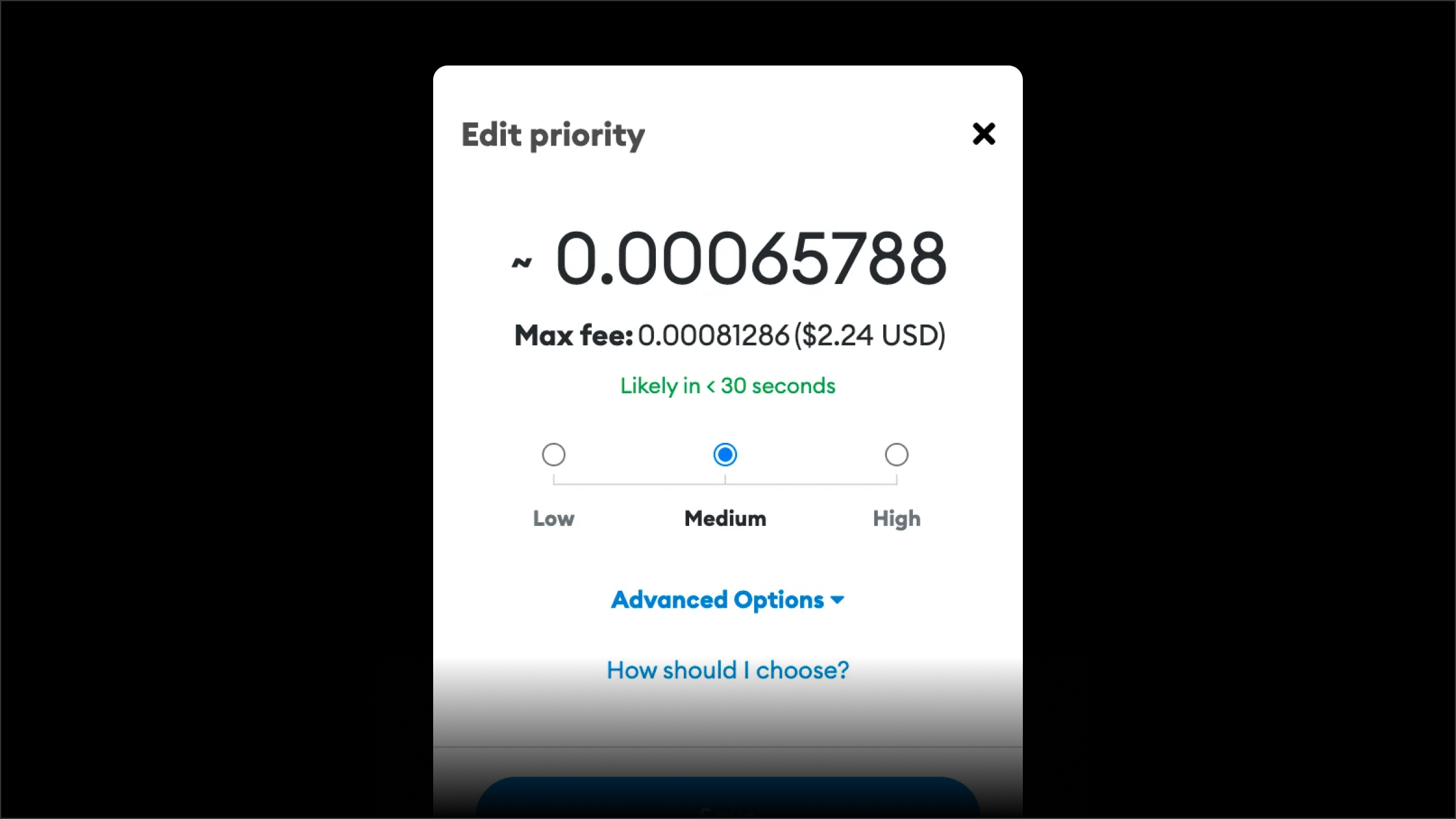
MetaMask's menu of posted prices for transaction priority fees.

At Ritual, we’re trying to enable the inclusion of transactions that require specialized computation (e.g. AI inference). While our fee mechanism Resonance has some nice properties (e.g. strategic simplicity, surplus-maximization, etc.), it still requires that people place bids. In this post, we look into whether a mechanism can be developed that solves the same problem while offering a posted-price experience. Although we reference Resonance, this post aims to be self-contained/doesn’t require the reader to have read previous posts. This post further generalizes far beyond transaction fee mechanisms, and discusses mechanism design within the general context of incentivizing distributed computing.

The main contribution of this post is a novel mechanism that theoretically works for any decentralized computing system, and determines the most economically valuable allocation of user requests to node resources, offering corresponding non-extractive posted prices to users and nodes that both parties would accept. There is a key difference between this mechanism and existing market mechanisms for decentralized computation: it obtains information regarding user valuations and node costs by making use of sophisticated third-party market-makers instead of relying on elicitation. Whereas market-makers on CLOBs are primarily responsible for simply setting posted prices for a traded asset, this mechanism incentivizes them to also find economically valuable allocations of requests to nodes.

TL;DR/Post contributions:

1. Defines the market-design problem for compute markets with general constraints (adapted from Resonance)
2. Gives a mathematical primer on some market design vocabulary
3. Presents a novel posted price mechanism that (i) picks the most economically valuable utilization of network compute resources given execution constraints (ii) selects pricing and node rewards that all parties will agree to, and (iii) selects pricing in a way that is not extractive, nor requires subsidies.

The sections labeled “Attempt 1” through “Attempt 3” can be skipped/skimmed for an abridged reading experience. These sections motivate the mechanism by walking through why simpler approaches wouldn’t work, beginning with a centralized market mechanism. Even if the market-makers have perfect information about demand and supply, incentivizing them to disclose this information is a highly nuanced problem.

Compute Markets with General Constraints

First, let’s outline the problem we’re trying to solve. In a compute market, users arrive with some compute requests $T$. These compute requests are to be executed by a set of nodes $N$. The goal of the market is to (i) figure out how to allocate compute requests to nodes (i.e. determine which nodes should execute which requests), and (ii) figure out payments: how much users should pay for receiving service and how much nodes should be paid for providing service. The catch is that there are complex constraints on how we’re allowed to allocate requests and nodes in (i).

In Ritual’s setting, the compute requests $T$ would correspond to transactions containing stateful precompiles that require specialized computation for execution (as discussed in previous Resonance posts). The nodes $N$ would correspond to specialized compute providers. There are several complex constraints in how we’re allowed to execute transactions on different nodes. For example, the nodes must have the hardware and software to support these transactions. Transactions that modify the same parts of the chain’s state also can’t be executed in parallel on different nodes, or else we’ll end up with an invalid state transition. In all, this makes Ritual’s block-building problem substantially more complicated than other L1s. In the Resonance posts, we called this market-design problem “The Heterogeneous Setting”.

Goal 1: Find an allocation.

Let’s dig a little deeper into the two goals of the market, focusing first on the allocation. In order to prove formal theorems about this market, we need some additional modeling. We define an allocation to be a map: $\alpha: T \to 2^N$ that specifies what subset of nodes in $N$ are responsible for executing each request. For example, if we want to allocate a request $t$ to be executed by node $n_1$, we’d consider an allocation $\alpha$ where $\alpha(t) = \{n_1\}$. If a compute request $t$ needs multiple nodes to execute (for example, if we want to redundantly compute $t$ on nodes $n_1$ and $n_2$ to get a better trust guarantee), then we’d consider an allocation $\alpha$ where $\alpha(t) = \{n_1, n_2\}$. We may also have a compute request $t$ that we can’t allocate because there aren’t any compatible nodes available. In that situation, we’d consider an allocation $\alpha$ where $\alpha(t) = \emptyset$.

Next, we need to model constraints on the allocation. Recall that in the setting we’re working in, we might have complex constraints beyond simple node compute capacity/gas constraints. We allow for general constraints $V$, where $V$ is a set of allocations $\alpha: T \to 2^N$, and enforce that the market must select a valid allocation $\alpha \in V$. We make no restrictions on $V$.

In Ritual’s setting we can encode node capacity constraints and hardware/software support constraints by only allowing allocations $\alpha$ to be in $V$ if, for each node $n \in N$, the bundle of transactions

allocated to $n$ under $\alpha$ can be executed by $n$. We can encode transaction hardware/software support constraints by only allowing allocations $\alpha$ in $V$ if the nodes $\alpha(t)$ that $t$ is allocated to are capable of executing $t$. More broadly, we can enforce that state conflicts do not occur, etc., by making the appropriate restrictions on $V$.

Goal 2: Determine pricing.

Next, let’s take a closer look at payments. The market needs to decide how much users should pay for service and how much nodes must receive for service. To formalize that, we define a request payment rule $\pi: T \to \R$ that specifies how much each request $t$ should pay for service, and a node payment rule $\phi: N \to \R$ that specifies how much each node $n$ should receive for providing service.

A Compute Market Instance

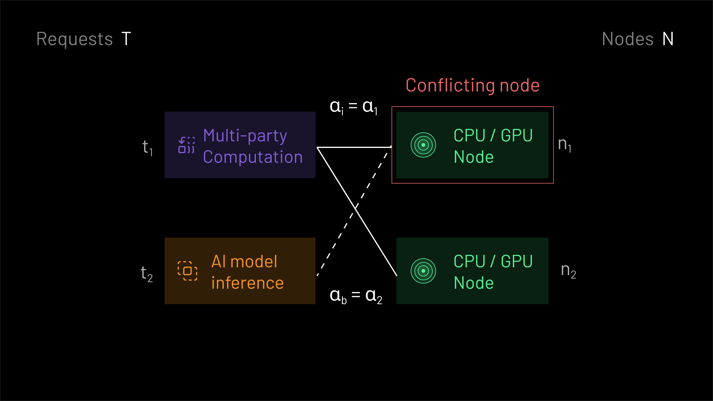
Now that we have some mathematical scaffolding to work with, we can take a look at an example of a market instance.

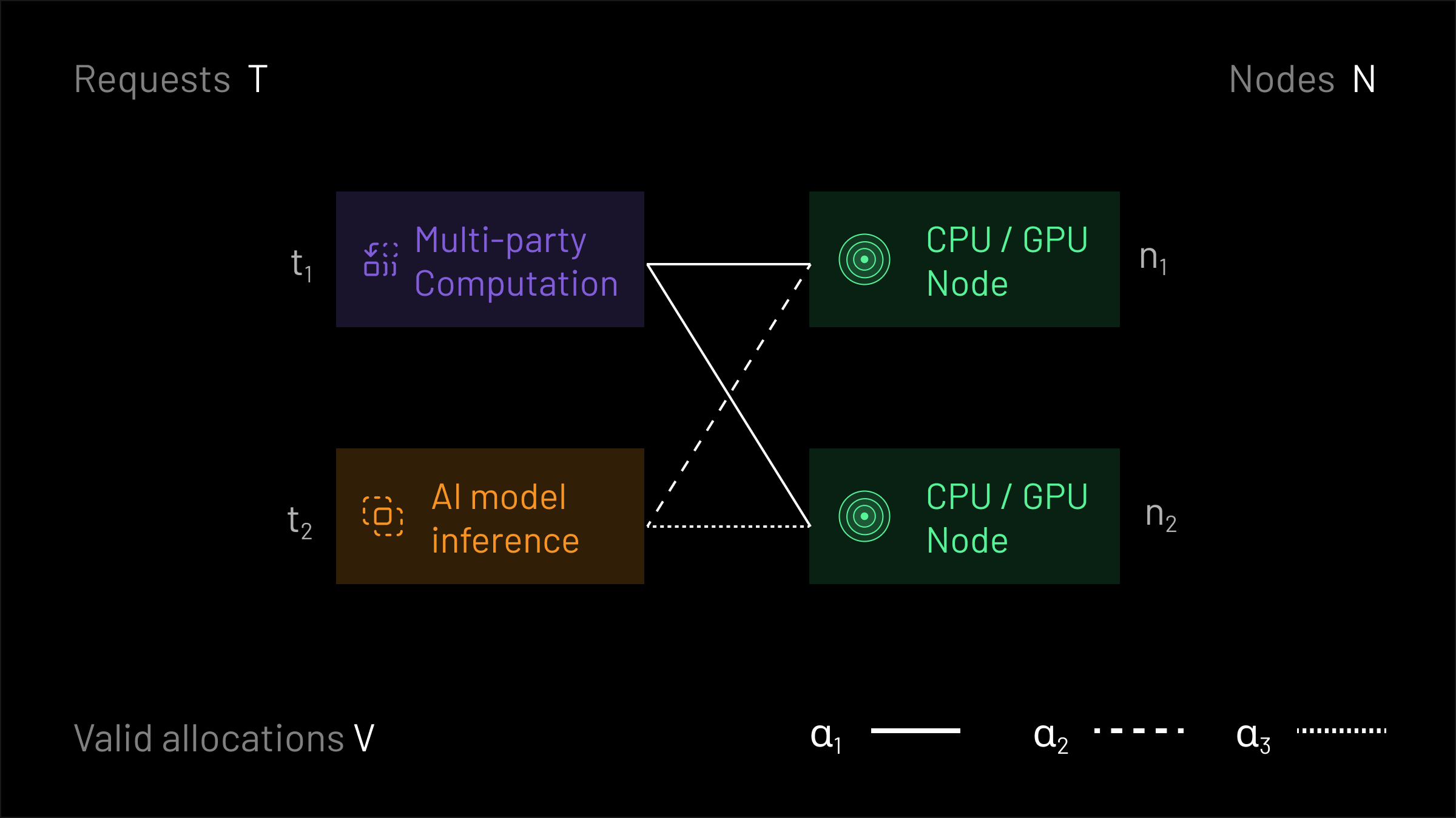
In this example, there are two requests $T = \{t_1, t_2\}$ and two nodes $N = \{n_1, n_2\}$. The request $t_1$ requires both nodes for valid execution, but the request $t_2$ may be executed on either one. A constraint exists that prevents any node from executing both requests. As a result, there are only four valid allocations $V = \{\alpha_\emptyset, \alpha_1, \alpha_2, \alpha_3\}$, where $\alpha_\emptyset$ allocates none of the requests, $\alpha_1$ allocates only $t_1$ to both nodes, $\alpha_2$ allocates only $t_2$ to node $n_1$, and $\alpha_3$ allocates only $t_2$ to node $n_2$. These allocations are notated formally below, and shown graphically in the image above.

To clear this market, we need to select one of the allocations $\alpha \in V$ within our valid collection of allocations, and select prices $\pi$ for the requests to pay and rewards $\phi$ for the nodes to receive. Furthermore, we’d like the experience for users submitting requests and nodes that are servicing requests to be a posted price experience— neither party should have to bid. But if all we cared about was meeting that desiderata, we might as well choose the allocation $\alpha_\emptyset$ and set all payments/rewards to zero. We’re missing a crucial second desiderata: that we’d like to select an economically efficient outcome. To make mathematical sense out of that, we need to introduce an economic model for market participants.

Market Participant Incentives

More concretely, we need to model the preferences of market participants. We adopt a simple model: for each compute request $t \in T$, the user who submitted it is willing to pay up to their valuation $v_t \ge 0$ for its execution. That is, if the price $\pi(t)\le v_t$ offered for executing $t$ is below or equal to the valuation for the request, then the user will choose to accept the offer (and will choose to reject the offer otherwise). Similarly, for each node $n \in N$, each node has a cost $c_n \ge 0$ which represents the lowest payment they’ll accept in exchange for service; if the reward offered $\phi(n) \ge c_n$ is greater than or equal to the node’s cost, then the node will choose accept the offer and provide service (and will choose to reject the offer otherwise).

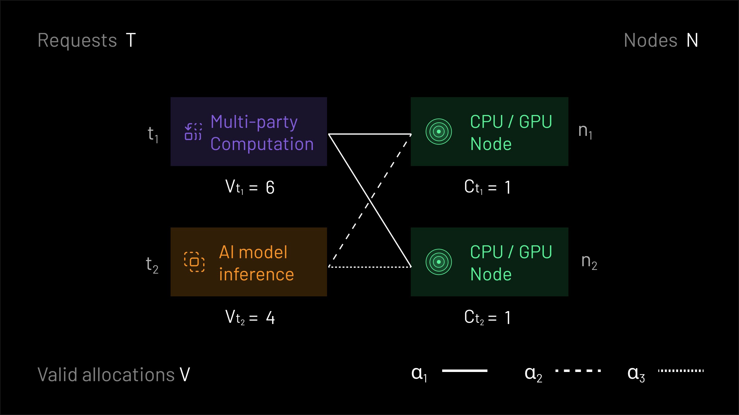
To make this concrete, let’s revisit our earlier example. Now, each of the requests has a valuation: $t_1$ is willing to pay at most $6$ tokens for service, and $t_2$ is willing to pay at most $4$ tokens for service. Similarly, each node has a cost: nodes $n_1$ and $n_2$ will accept any offer that pays at least $1$. Recall that as before, there are three non-null allocations that are valid in this example: $V = \{\alpha_\emptyset, \alpha_1, \alpha_2, \alpha_3\}$.

Utilities

Let’s take a closer look at the preferences of our market participants. Users will accept an offer for service for a request $t$ if their payment is less than their valuation $\pi(t) \le v_t$. But there’s more richness here: if given the choice between two offers for service where one is cheaper than the other, a user will prefer the cheaper option. We can write down the utilities of each market participant, which represents the amount of value in tokens that the participant gains (or loses) from their interaction with the market. The utility of a user submitting a request $t$ under an allocation $\alpha$ and payment rule $(\pi, \phi)$ can be modeled as

Going back to our example, recall that $t_2$ was willing to pay at most $4$ tokens for service. Suppose we clear the market under the allocation $\alpha_2$ and set $\pi(t_2) = 2$ tokens. Since $t_2$ is allocated under $\alpha_2$ (as $\alpha_2(t_2) = \{n_1\} \ne \emptyset$), the utility that $t_2$ obtains is equal to

tokens. These $2$ tokens of value represent the economic surplus that $t_2$ received by participating in the market. Suppose we set $\pi(t_1) = 0$ under the same allocation $\alpha_2$. Since $t_1$ is not allocated under $\alpha_2$ (as $\alpha_2(t_1) = \emptyset$), the utility that $t_1$ obtains is equal to $0 - 0 = 0$ tokens.

What about the utility for nodes? Returning to our simple model, a node $n$ will accept an offer to provide service if their reward exceeds their cost $\phi(n) \ge c_n$. Further, if given the choice between two offers to provide service where one pays more than another, the node will prefer the option that pays more. As such, we model the utility of a node $n$ under an allocation $\alpha$ and payment rule $(\pi, \phi)$ as

In our running example, suppose that we again select the allocation $\alpha_2$ and set $\phi(n_1) = 2$. Since $n_1$ is allocated under $\alpha_2$ (as $\alpha_2^{-1}(n_1) = \{t_2\} \ne \emptyset$), the utility that $n_1$ obtains is equal to

token. Suppose that we set $\phi(n_2) = 0$ again under the allocation $\alpha_2$. Since $n_2$ is not allocated under $\alpha_2$ ($\alpha_2^{-1}(n_2) = \emptyset$), the utility $n_2$ obtains is equal to $0 - 0 = 0$ tokens.

As an aside, our model for node costs without loss of generality extends to the case where nodes may face different costs for different workloads. This is because we can set arbitrary validity sets $V$; to represent a node that faces different costs across different workloads, we can simply instantiate multiple nodes, where a valid allocation can only allocate to one of these instantiations. Each instantiation has a different cost, and a different collection of valid requests that it can service.

Individual Rationality

We can now relate these definitions for the market participants’ utilities to the simple model we described earlier. If a user submitting a request $t$ is given an offer for service such that $\pi(t) \le v_t$, then that offer for service corresponds to an allocation $\alpha$ such that $\alpha(t) \ne \emptyset$. As such,

Similarly, if a node is offered a reward $\phi(n) \ge c_n$ in exchange for service, then that offer corresponds to an allocation $\alpha$ such that $\alpha^{-1}(n) \ne \emptyset$. Accordingly,

The converse of these statements is also true: if a user submitting a request obtains non-negative utility, then they must have received service at a price that is at most their valuation. If a node providing service obtains non-negative utility, then they must have been offered a reward that exceeds their cost. Market participants will accept an allocation $\alpha$ with payment rule $(\pi, \phi)$ if all participants have non-negative utility. If this holds true, then we call $(\alpha, \pi, \phi)$ individually rational. If the mechanism returns an allocation and pricing that is not individually rational, then participants will not choose to use the mechanism.

Returning to our running example, let’s suppose that we indeed have chosen the allocation $\alpha_1$. Let’s run through some example payment rules:

Under $\alpha_1$, we can see that the payment rule $(\pi_1, \phi_1)$ is not individually rational, since

It violates individual rationality a second time, since

All three payment rules $(\pi_2, \phi_2)$, $(\pi_3, \phi_3)$ and $(\pi_4, \phi_4)$ are individually rational under $\alpha_1$. That is, the market would clear the allocation $\alpha_1$ if the prices $(\pi_2, \phi_2)$, $(\pi_3, \phi_3)$, or $(\pi_4, \phi_4)$ were offered to users and nodes.

Aggregate Utility

The previous definitions aimed to characterize the preferences of individual market participants. Ideally, we would like to be able to say something about our market mechanism providing good aggregate outcomes for all of the market participants. Just like how we defined a utility function for each individual, let’s think about how we might define an analogue of a utility function for the entire market. We’ll use these aggregate definitions to develop a principled way for accomplishing our two goals of choosing an allocation and determining payments.

Welfare

Recall that in our model for each individual’s utility, there were two terms that were added (or subtracted) together. One term indicated how much value the market participant got from the allocation — in the case of requests this was their valuation (maximum willingness to pay) and in the case of nodes this was their cost (minimum reward to provide service). The other term offset the individual’s utility based on the payment rule, reducing the individual’s utility by a payment (in the case of a request) or increasing the individual’s utility by a reward (in the case of a node).

Let’s focus on the first term that depends only on the allocation. We call the aggregate analogue of this term welfare. Welfare $\mathcal W: V \to \mathbb R$ is formally defined as

Welfare measures the total value (in tokens) generated by an allocation $\alpha$ by adding up the valuations of all allocated requests and subtracting the costs of all allocated nodes; we may charge users in aggregate up to $v_t$ for each user whose request was allocated and have them take the offer, but we only need to pay out a minimum of $c_n$ for each node providing service, generating $\mathcal W(\alpha)$ in net value. Another way to think about $\mathcal W(\alpha)$ is that market participants, in aggregate, are willing to pay $\mathcal W(\alpha)$ for trade to take place under the allocation $\alpha$.

We can compare allocations on the basis of the welfare they generate for market participants. As a concrete example, below we compute the welfare for each of the allocations in our running example:

We can see that the allocation $\alpha_1$ is the most economically valuable out of the valid allocations, so we’d ideally like the market mechanism to select it. That takes care of our first goal we had for our market mechanism of finding an allocation, but how should we set payments?

Margin

Clearly, we would like our payment rules to be individually rational under the allocation that we select, otherwise market participants will choose not to participate in the market mechanism. But even though they’re all individually rational, are the payment rules $(\pi_2, \phi_2)$, $(\pi_3, \phi_3)$, and $(\pi_4, \phi_4)$ that we defined earlier all equally good?

To devise a more principled method for setting payments, let’s now try to think of an aggregate form of the other term in an individual’s utility that keeps track of the offset due to request’s payment or node’s reward. We can define the margin of a payment rule $(\pi, \phi)$ as

The margin keeps track of how much more (or less) was collected from users by the marketplace in fees relative to what was paid out to nodes as rewards. Ideally, we’d like to select a payment rule that neither extracts money from users nor requires a subsidy from the market in order for trade to take place.

Let’s compute the margins of each of the payment rules:

Notice how $(\pi_2, \phi_2)$ has a positive margin and is thus extractive— more money is taken from users than is paid out to nodes. Although $\mathcal W(\alpha_1) = 4$ tokens of value are generated by the allocation $\alpha_1$, the users and nodes only get to “keep” 3 of those tokens, since the market takes a margin of $1$ token under this payment rule.

Conversely, notice that the payment rule $(\pi_4, \phi_4)$ has a negative margin and is thus not budget-balanced— more money is paid out to nodes than is taken from users. As a result, the marketplace is subsidizing trade by $1$ token, which may not be sustainable in the long-run.

Payment rules $(\pi_1, \phi_1)$ and $(\pi_3, \phi_3)$ are both non-extractive and budget-balanced. In particular, $(\pi_3, \phi_3)$ is the only payment rule of these four that is individually-rational, non-extractive, and budget-balanced.

Surplus

Now let’s put everything together to get the full form of aggregate utility, which we’ll call surplus. We defined welfare and margin to be aggregate forms of the two terms that make up each individual’s utility. Let’s make that intuition precise. Formally, the surplus

is given by the welfare minus the margin. This looks very similar to the utility function we wrote down for each individual: the first term represents the total economic value generated from trade, and the second term offsets that by any payments that are made in aggregate to the marketplace. Expanding, we can also rewrite the surplus as

In other words, the surplus is exactly equal to the sum of all market participants’ utilities, and therefore denotes the total willingness to pay the market has for the option provided by the market.

We would ideally like to accomplish our two goals of finding an allocation and determining payments/rewards in a way that is individually rational and maximizes surplus.

Claim: An allocation and budget-balanced payment rule $(\alpha, \pi, \phi)$ maximizes surplus if and only if $\alpha$ maximizes welfare and $(\pi, \phi)$ has zero margin.

Intuition: Since the payment rule is budget-balanced, it can’t have a negative margin. Therefore, any $(\alpha, \pi, \phi)$ with $\alpha$ welfare-maximizing and $(\pi, \phi)$ with zero margin must be surplus-maximizing. Furthermore, for any allocation, there’s a way to make a zero margin payment rule, by simply setting node rewards $\phi(n) = \sum_{t \in \alpha^{-1}(n)}\pi(t)$ equal to the sum of the payments that the requests allocate. Therefore, any surplus-maximizing $(\alpha, \pi, \phi)$ must have $\alpha$ as welfare maximizing, else we could increase surplus by choosing a higher welfare allocation and selecting a zero-margin payment rule.

Designing a Posted-Price Market Mechanism

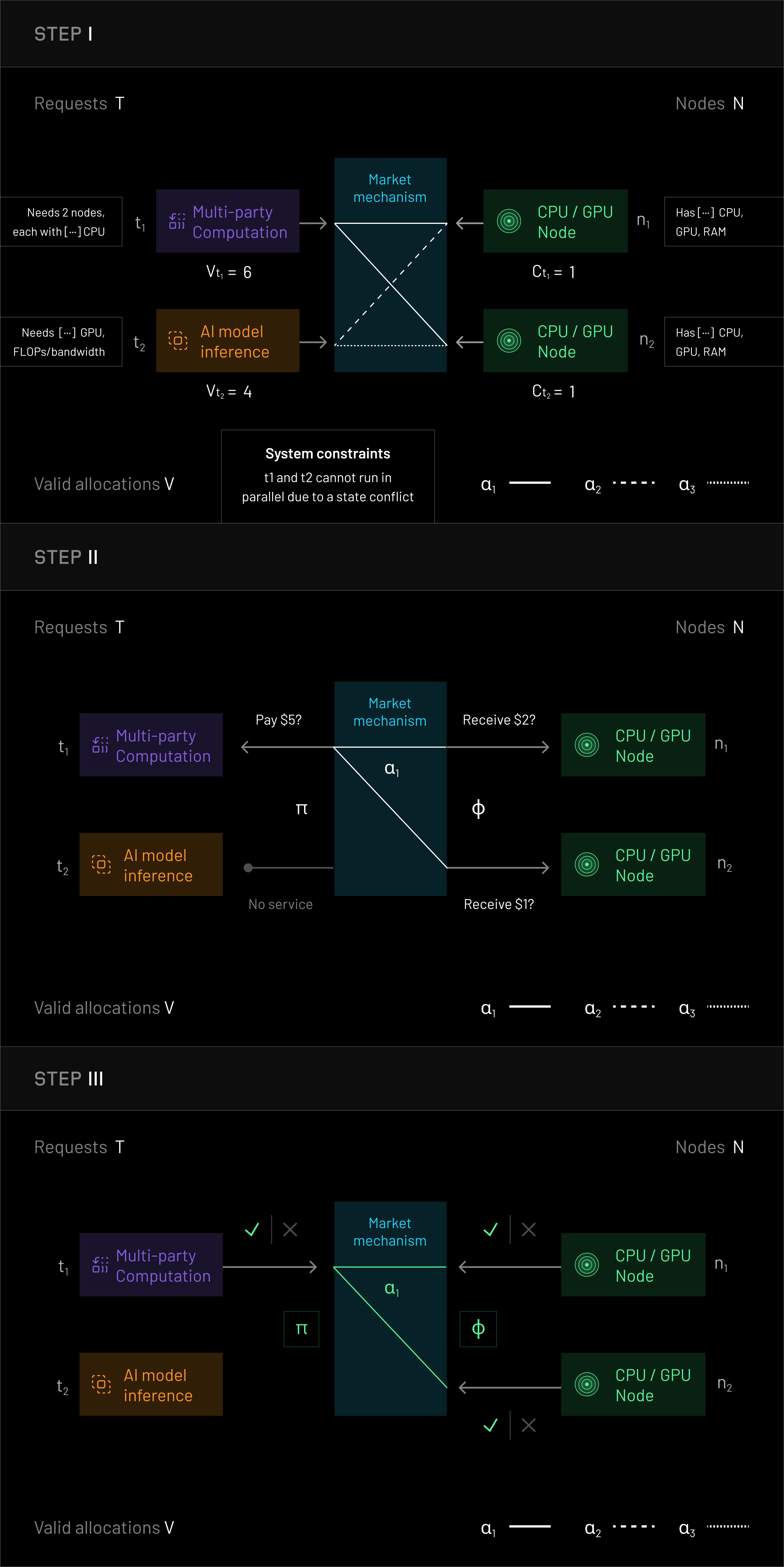
Now that we have all of those primitives under our belt, we can return to the original problem: designing a posted-price mechanism for a compute market with general constraints. The end-to-end flow that we’re shooting for is as follows:

1. Users submit requests and corresponding execution constraints. Nodes submit execution constraints. These (and additional system-wide constraints) are aggregated into a set $V$ of valid allocations.
2. The market mechanism selects a valid allocation $\alpha \in V$ and a payment rule $(\pi, \phi)$. Prices and allocation results are then served to users
3. Users and nodes choose to either accept or reject the allocation results at the prices specified by the payment rule.

The meat of this problem is in the second step. Concretely, given a set of valid allocations $V$, We would like to select an allocation rule $\alpha$ and payment rule $(\pi, \phi)$ that satisfy two properties:

Surplus Maximization: The allocation and payment rule $(\alpha, \pi, \phi)$ should maximize surplus, or the economic value that is distributed to the market participants.

Individual Rationality: The payment rule $(\pi, \phi)$ should be individually rational under $\alpha$ so that in step 3, all parties agree to the allocation and payments selected by the mechanism, and the market clears.

Using the intuition we developed in the previous section, we may equivalently require that the the below three conditions are met; it’ll sometimes be useful to refer back to this in our subsequent analysis:

Welfare Maximization: The allocation $\alpha$ should be maximal in terms of the economic value $\mathcal W(\alpha)$ it generates.

Zero Margin: The marketplace should neither be extractive, nor should it require subsidies for trade to occur. That is, the margin $\mathcal M(\pi, \phi)$ of the payment rule should be equal to zero.

Individual Rationality: The payment rule $(\pi, \phi)$ should be individually rational under $\alpha$ so that in step 3, all parties agree to the allocation and payments selected by the mechanism, and the market clears.

Crucially in this flow, users and nodes do not ever submit bids or otherwise signal their valuations or costs. So how can we compute a good allocation $\alpha$ and payment rule $(\pi, \phi)$ without any information?

Attempt 1: Centralized Routing

With truly no information about valuations and costs, it’s clearly impossible to find the most economically valuable allocation and set prices appropriately. To resolve this, we introduce an informed market-maker (referred to as a broker in previous posts) whose job it is to set a good allocation and payment rule. In what follows, we’ll assume that the market-maker is a profit-maximizing entity with perfect information. The idea behind assuming perfect information is (i) simplicity of analysis, and (ii) to understand what happens in the limit case when the market-maker becomes highly sophisticated (e.g. as has occurred in established centralized matching markets like Uber).

A straight-forward approach for clearing the market that is used by many centralized online marketplaces looks something like the below mechanism:

Let’s go back to our running example to see how this market mechanism would work. Which allocation would the market-maker select? We’ll begin by supposing that the market-maker selected allocation $\alpha_1$. Now we can try to see what the market-maker would charge to maximize profit. In allocation $\alpha_1$, request $t_1$ is allocated to both $n_1$ and $n_2$. Since request $t_2$ is not allocated, the market-maker must set $t_2$’s payment $\pi(t_2) = 0$, or else $t_2$ will reject the offer. To maximize the margin $\mathcal M(\pi, \phi)$, the market-maker should charge $t_1$ as much as possible, and pay as little as possible to the nodes. Since $t_1$ has a valuation of $6$, and won’t accept any offer that charges more than that, we should correspondingly set $\pi(t_1) = v_{t_1} = 6$. Similarly, we should set $\phi(n_1) = c_{n_1} = 1$ and $\phi(n_2) = c_{n_2} = 1$. This yields a total margin of $\mathcal M(\pi, \phi) = 6 - 1 - 1 = 4$. Notice that this is equal to the welfare of $\alpha_1$. If the market-maker were to choose $\alpha_2$ or $\alpha_3$, the most that could be extracted in margin would be $\mathcal W(\alpha_2) = \mathcal W(\alpha_3) = 3$.

Theoretical Analysis

Let’s try to generalize what happened in the previous example. Recall that we’ve assumed that the market-maker is profit-maximizing and has perfect information. We can deduce the properties of the final allocation and payment rule using the following key claim:

Claim: Fixing a specific valid allocation $\alpha$, the market-maker maximizes profit by charging each request equal to the request’s valuation (if allocated)

and paying each node its cost (if allocated)

The total profit the market-maker receives $\mathcal M(\pi, \phi) = \mathcal W(\alpha)$ is equal to the welfare of the allocation.

Intuition: Supposing that the market-maker has committed to selecting some particular allocation $\alpha \in V$, the market-maker can maximize their margin $\mathcal M(\pi, \phi)$ by charging users as much as possible and paying nodes as little as possible. The market-maker can’t charge an arbitrarily large amount of money, or else the users and nodes won’t accept the offer. The most the market-maker can charge while having users accept the offer is $v_t$ if the request is allocated (i.e. $\alpha(t) \ne \emptyset$), or $0$ in the case that the request is not allocated. Similarly, the least that the market-maker can pay out to the nodes is $c_n$ if the node is allocated (i.e. $\alpha^{-1}(n) \ne \emptyset$) or $0$ if the node is not allocated. This yields the payment rules $\pi(t) = 1[\alpha(t) \ne \emptyset] \cdot v_t$ and $\phi(n) = 1[\alpha^{-1}(n) \ne \emptyset] \cdot c_n$ as claimed. We can now compute the total margin that the market-maker makes as

Mechanism Properties

We can now go through each of our desired properties:

Attempt 2: Competing Market-Makers

To get a better market mechanism, we need to fix the fact that the central market-maker extracted all of the gains from trade. A natural way to do this is to introduce competition. Instead of having just one market-maker, what if we introduce additional market-makers to compete? Let’s modify the mechanism to allow multiple market-makers to submit proposals. Now we need some way of having the market mechanism decide which proposal to accept. The simple solution to drive margins to zero would be to select the proposal with the lowest margin:

Now let’s try to reason about how this mechanism behaves, returning to our running example. We saw that if there was just one market-maker, then the mechanism would select the allocation $\alpha_1$ and choose payments $(\pi, \phi)$ that would charge $t_1$ her valuation $v_t = 6$ and pay nodes $n_1$ and $n_2$ their costs $c_{n_1}$ and $c_{n_2}$ respectively, to obtain a margin $\mathcal M(\pi, \phi) = 4$. What happens when we add a second market-maker?

Competing with a fixed allocation

First, let’s suppose that both market-makers (let’s call them Alice and Bob) are forced to choose the allocation $\alpha_1$. We’ll reason about the final payment rule that will be selected by the mechanism. Given that we’ve already assumed that Alice and Bob have chosen the allocation $\alpha_1$ (and that this is common knowledge), Alice and Bob’s choices are restricted to selecting a payment rule. Neither Alice nor Bob would choose a payment rule $(\pi, \phi)$ that has negative margin $\mathcal M(\pi, \phi) < 0$, or else they’ll lose money in the case that they win.

Now let’s think about things from Alice’s perspective. Let’s suppose that Bob has chosen a payment rule $(\pi', \phi')$. What payment rule $(\pi, \phi)$ should Alice choose as a best response? Alice wouldn’t want to violate the individual rationality constraints or else if she wins, then she’ll have to pay a penalty of $\gamma$. Next, suppose that Bob’s margin $\mathcal M(\pi', \phi')$ > 0. Alice can’t win with any margin greater than Bob’s. Thus, Alice should choose an individually rational payment rule $(\pi, \phi)$ where $\mathcal M(\pi, \phi)$ is just a tad less than Bob’s margin $\mathcal M(\pi', \phi')$ so that her submission will beat Bob’s and she can extract the largest possible margin.

But from Bob’s perspective, things look the same! He also wants to undercut Alice’s margin by just a tad so that he wins and can extract the largest possible margin. As a result, the only joint strategies of Alice and Bob where neither wants to change their strategy (i.e. pure Nash equilibria) are those in which one of the two has selected an individually rational proposal with zero margin. So does that mean we’ve solved the problem?

Competing without a fixed allocation

Unfortunately, not quite. Our whole analysis hinged on Alice and Bob being forced to select $\alpha_1$. But how would we force them to do this? Remember, in our model, the market-makers are assumed to have perfect information about the valuations and costs of the requests and nodes. However, the market mechanism itself does not have any such information. There’s no way for the mechanism to know that $\alpha_1$ was the most economically valuable allocation. In the centralized case, this didn’t matter, since the market-maker was incentivized to choose the most economically valuable allocation so that she could extract as much as possible. With competing market-makers, however, nothing stops Bob from choosing the null allocation $\alpha_\emptyset$ and setting all payments $\pi'(t) = 0$ and all rewards $\phi'(n) = 0$. Indeed, that payment rule has margin $\mathcal M(\pi', \phi') = 0$ and would therefore outcompete any proposal that Alice makes (assuming ties are arbitrarily broken in favor of Bob).

Mechanism Properties

In net, this mechanism achieves the following properties (assuming there are at least $2$ market-makers):

A General Template

We tried to fix the extractive properties of the centralized mechanism by introducing competition (and succeeded) but it potentially costs us all gains from trade. So where did we go wrong? To understand that, let’s contextualize the previous mechanism in terms of a more general sequential template:

This general type of mechanism iterates through the market-makers’ proposals and keeps in memory a “current best” proposal. For each proposal, it checks whether the proposal is an improvement over the current best, as determined by the $\textbf{IMPROVEMENT}$ function. If the proposal is indeed an improvement, then it replaces the “current best”.

The minimum margin mechanism can be written as a sequential improvement mechanism by setting $\textbf{IMPROVEMENT}(b, i)$ to compare the margins of the two proposals (i.e. return $\text{TRUE}$ if $\mathcal{M}(\pi_i, \phi_i) < \mathcal{M}(\pi_b, \phi_b)$). The problem with this (as we demonstrated above) is that this improvement test proved to be faulty: it returns $\text{TRUE}$ even in cases when the proposal from market-maker $i$ yields lower surplus than that of $b$, since it is possible for $i$ to be lowering the margin for an allocation that is less economically valuable (i.e. has lower welfare).

In what follows, we’ll try to come up with a better mechanism within this template by designing a better test for improvement.

Attempt 3: Sequential Pareto Improvements for Conflicts

When we’re assessing the next market-maker’s proposal, there are two cases to consider. First, it’s possible that there are no conflicting requests or nodes between the current best $b$’s proposal and market-maker $i$’s proposal. In this case, there’s nothing wrong with running both proposals concurrently (and indeed one would do this if this mechanism were to be implemented in practice). For simplicity of analysis, we’re going to instead ignore market-maker $i$’s proposal and keep $b$’s proposal, since market-maker $i$ could have just included the contents of $b$’s proposal in its own proposal.

This leaves us with only the second case, where market-maker $i$’s proposal conflicts with $b$’s proposal. Which proposal should win? At a high-level, in this attempt we’re going to see what happens if we let the conflicting market participants decide which proposal wins.

Conflicting Requests and Nodes

To understand what’s going on here, let’s think about things a bit more formally. Let’s consider the two different proposals $(\alpha_i, \pi_i, \phi_i)$ and $(\alpha_b, \pi_b, \phi_b)$ made by market-maker $i$ and $b$ respectively. We’ll define $T_i$ and $N_i$ to be the requests and nodes that are allocated under $\alpha_i$.

We’ll similarly define

to be the requests and nodes that are allocated under $\alpha_b$. To compare the different market outcomes, it’s helpful to consider three different groups of market participants:

The first group consists of “conflicting” market participants: these are requests and nodes that were allocated under both $\alpha_i$ and $\alpha_b$.

The next group consists of requests $T_i \setminus C_T$ and nodes $N_i \setminus C_N$ that were allocated under the allocation $\alpha_i$ but not under $\alpha_b$. The third and final group consists of requests $T_b \setminus C_T$ and nodes $N_b \setminus C_N$ that were allocated under $\alpha_b$ but not under $\alpha_i$.

We can decompose the surplus generated by the two proposals in terms of the contribution that’s given by the conflicting requests and nodes and the contribution that’s given by the non-conflicting requests and nodes:

For convenience, we’re using the notation $\mathcal S(i) := \mathcal S(\alpha_i, \pi_i, \phi_i)$ as shorthand for the surplus generated by market-maker $i$’s proposal. Similarly, we’re using $u_t(i) := u_t(\alpha_i, \pi_i)$ and $u_n(i) := u_n(\alpha_i, \phi_i)$ as shorthand for the request and node utilities.

If we were to write $\mathcal S(b)$ in the same way, we can see that the difference in surplus between the two proposals depends only on the relative surplus of the non-conflicting participants:

If $\alpha_i$ were indeed a higher welfare allocation than $\alpha_b$, then that means that the non-conflicting market participants that are allocated under $\alpha_i$ are willing to pay more in aggregate for allocation than those under $\alpha_b$. We’ll use this insight to make a new $\textbf{IMPROVEMENT}$ function!

Pareto Improvements for Conflicting Requests and Nodes

To convert that intuition into an $\textbf{IMPROVEMENT}$ function, we’ll take some inspiration from the welfare theorems of economics: if the non-conflicting market participants of $\alpha_i$ are indeed willing to pay more in aggregate for allocation than those under $\alpha_b$, then there should be a way for market-maker $i$ to set the payments $(\pi_i, \phi_i)$ so that every conflicting **market participant strictly prefers the market outcome $(\alpha_i, \pi_i, \phi_i)$ to the market outcome $(\alpha_b, \pi_b, \phi_b)$.

Concretely, we let $\textbf{IMPROVEMENT}(b,i)$ be equal to $1$ if

and equal to $0$ otherwise. An interpretation of this condition is that market-maker $i$ offers a cheaper price for every conflicting request and a greater reward for every conflicting node. If this is true, then we know that every conflicting market participant prefers the market outcome proposed by market-maker $i$ to that proposed under the “current best” market-maker $b$ regardless of their valuations and costs (which remain unknown to the market mechanism).

Since a formal proof would make this blog post even more dense than it already is, we now show informally by an example that if a market-maker intends to offer an outcome with higher surplus than the current best market-maker, then there exists a way to set payments such that it satisfies this $\textbf{IMPROVEMENT}$ function.

Claim: Suppose that market-maker $i$ would like to propose an allocation $\alpha_i$ and extract a margin $m$. If the surplus of this outcome will exceed that of the current best, i.e. $\mathcal W(\alpha_i) - m > \mathcal S(\alpha_b, \pi_b, \phi_b)$, then there exists a budget-balanced and individually rational payment rule $(\pi_i, \phi_i)$ for $\alpha_i$ such that every conflicting market participant strictly prefers the market outcome $(\alpha_i, \pi_i, \phi_i)$ over the outcome $(\alpha_b, \pi_b, \phi_b)$ (i.e. $\textbf{IMPROVEMENT}(b,i) = 1$).

Intuition: Let’s walk through what this statement means and the intuition behind it using our running example.

Suppose that the current best proposal uses the allocation $\alpha_b := \alpha_2$, with a payment rule $(\pi_b, \phi_b)$ that extracts no margin. For concreteness, let’s suppose that the rule charges $\pi_b(t_2) = 4$ from $t_2$ and pays out $\phi_b(n_1) = 4$ to $n_1$. Next, suppose that market-maker $i$ would like to propose the allocation $\alpha_i := \alpha_1$. There are no conflicting requests between $\alpha_i$ and $\alpha_b$, but since $\alpha_i$ allocates to both nodes, there is a conflicting node: $n_1$. Let’s further suppose that market-maker $i$ would like to further extract a margin of $\frac12$. Does an individually rational and budget-balanced payment rule $(\pi_i, \phi_i)$ exist such that it extracts a margin of $\frac12$ and the conflicting node $n_1$ prefers it strictly to the current best proposal? According to our claim, we should first compare

As the surplus that the second market-maker aims to achieve is higher than the surplus attained by the first market-maker, our claim states that there should exist a payment rule that the second market-maker can apply that would attain that surplus, and have the conflicting node $n_1$ strictly prefer the proposal to the one made by the first market-maker.

Let’s try to find such a payment rule. Under the current best proposal, node $n_1$ is being paid $\phi_b(n_1) = 4$. The request $t_1$ is willing to pay up to $v_{t_1} = 6$. So to outcompete the current best proposal, we can set $\phi_1(n_1) = 4\frac12$. The node $n_2$ has a cost $c_{n_2} = 1$, so the market-maker $i$ must pay out at least this much for the payment rule to be individually rational. Let’s set $\phi_i(n_2) = 1$ to satisfy this requirement. Finally, we must extract $\frac12$ as a margin. It is possible to do this by setting $\pi_i(t_1) = 6$, noting that this payment is also individually rational. Thus, we were able to find the payment rule as guaranteed by the claim. We could have done this no matter what payment rule was set by the current best market-maker.

This intuition leads us to the following mechanism:

This is exactly the Sequential Improvements mechanism with the $\textbf{IMPROVEMENT}$ function described above.

Informal Analysis

We’ll try to informally understand how the mechanism behaves by running through what an iterated sequences of best responses might look like on our running example. Let’s start by supposing that there are two market-makers, and that the ordering chosen by the market mechanism has market-maker $1$ proposing the allocation $(\alpha_2, \pi_1, \phi_1)$ where $\alpha_2$ is as defined in our running example (it maps request $t_2$ to the node $n_1$). What should market-maker $2$ do? One way that market-maker 2 could try to win while maximizing profit is to propose the same allocation $\alpha_2$ that market-maker 1 proposed, but tighten all of the prices to slightly reduce the margin. As this proposal provides better prices for all conflicting requests and nodes (i.e. the same request $t_2$ and node $n_1$ that were allocated under $\alpha_2$), it would replace market-maker 1’s proposal as the current best. Now, market-maker 2 will win with a payoff that is just a hair less than what market-maker 1 would have received if he were to win instead.

But is that the best that market-maker 2 can do? What if market-maker 2 instead proposed the allocation $\alpha_1$? Because $\alpha_1$ has a higher welfare of 4 relative to the welfare 3 of $\alpha_2$, market-maker 2 can actually get a bigger cut by proposing this allocation while still offering better terms to every conflicting market participant (in this case, node $n_1$). This is because request $t_1$ is simply willing to pay more, even accounting for the added cost that must be paid to node $n_2$. This follows from the claim we made earlier.

How should market-maker 1 respond to this? Since $\alpha_1$ is the allocation with the highest welfare, we should expect that market-maker 1 would simply repropose the same allocation with a tightened margin. Market-maker 2 would then do the same thing, until the iteration leads to the margin being driven to zero. If that were to take place, we’d end up with the highest welfare allocation being chosen with zero extracted margin, leading to the outcome we desired…right?

Unstable Best-Response Dynamics

Unfortunately, our market mechanism doesn’t quite lead to the desirable outcome. Let’s go back to when we considered market-maker 1’s best response after market-maker 2 proposed $\alpha_1$. As it turns out, no matter what payment rule market-maker 2 sets, market-maker 1 will be able to win by proposing either $\alpha_1$ or $\alpha_3$, despite the fact that both of these allocations actually yield less welfare. Let’s take a look at why this happens:

Suppose that market-maker 2 begins by proposing the payment rule $(\pi_2, \phi_2)$ under the allocation $\alpha_2$. Because this payment rule is individually rational (market-maker 2 will have to pay a penalty $\gamma$ if the match fails), we know that the total incoming payment $\pi_2(t_1)$ is at most $t_1$’s valuation $v_{t_1} = 6$. Furthermore, since the payment is budget-balanced (since market-maker 2 will lose money if trade is subsidized), this means that $\phi_2(n_1) + \phi_2(n_2) \le 6$. In particular, this means that market-maker 2 cannot pay both $n_1$ and $n_2$ at least $4$, since $4 + 4 = 8$. If market-maker 2 pays $n_1$ less than $4$, then market-maker 1 can propose the allocation $\alpha_2$ that matches $t_2$ to $n_1$, and since $t_2$ is willing to pay up to $v_{t_2} = 4$, market-maker 1 can find an individually rational and budget balanced payment rule that offers better terms to the conflicting node $n_1$. If instead market-maker 2 pays $n_2$ less than $4$, then market-maker 1 can similarly propose the allocation $\alpha_3$ that matches $t_2$ to $n_2$ and find corresponding payments that offer $n_2$ better terms. Furthermore, since market-maker 2 can’t even pay both $n_1$ and $n_1$ more than $3$, market-maker 1 will be able to make a margin of at least $1$ on this proposal.

However, after market-maker 1 makes this proposal, market-maker 2 can again best-respond by selecting the allocation $\alpha_1$ again, but with different payments (this follows from the same argument we made earlier). In net, the sequence of allocations under iterated best responses will keep bouncing back and forth between the welfare-maximizing allocation $\alpha_1$ and one of $\alpha_2$ or $\alpha_3$.

Mechanism Properties

In net, this mechanism achieves the following properties (assuming there are at least $2$ market-makers):

Attempt 4: Sequential Pareto Improvements with Tolerances

We were close with the last mechanism. If we are able to somehow fix the unstable best-response problem, then we can indeed have all three properties. In our final attempt, we show how this can be done by introducing tolerances.

At a high level, the core problem comes from the fact that our earlier claim is not an “if and only if” statement. We walked through how if one market-maker intends to make a proposal with higher surplus than another market-maker, then there indeed exists a payment rule they can set along with the allocation that will replace the former market-maker’s proposal. The problem is that the other direction may not hold: as we saw in our running example, it can be possible to replace a former market-maker’s proposal (i.e. have $\textbf{IMPROVEMENT}(b,i) = 1$) even if the new proposal yields lower surplus. As a result, we may find ourselves with an unstable outcome. In order to fix this, we need to modify our replacement rule to something that does function as an “if and only if”. In particular, we need to be more conservative with our replacement rule, as we were allowing proposals with higher surplus to be replaced.

Constructing a Perfect Test for Improvement

Suppose that there are two market-makers, and market-maker 1 wishes to set an allocation $\alpha_1$ and extract a total margin $m_1$. Similarly, market-maker 2 wishes to set an allocation $\alpha_2$ and extract a total margin $m_2$. Assuming both market-makers propose individually rational payments, can we perfectly determine which market outcome will yield greater surplus? Our previous claim yielded a one-sided test. If market maker 1’s surplus $\mathcal W(\alpha_1) - m_1$ exceeds that of market-maker 2, $\mathcal W(\alpha_2) - m_2$, then there exists a way for market-maker 1 to set payments such that every conflicting request and node is offered better terms under market-maker 1’s proposal than market-maker 2’s proposal. However, the converse of that statement was not true. As illustrated in the example above, even though the allocation $\alpha_2$ with an extracted margin of $1$ yields less surplus than the allocation $\alpha_1$ with an extracted margin of, let’s say, $\frac12$, it is still possible to set the new allocation to $\alpha_2$ while offering better terms to the conflicting node.

Introducing Tolerances

To resolve this issue, we’re going to allow the market-makers to estimate what the surplus of their proposal is. We can’t simply have the market-makers provide non-binding estimates, however, or else they will claim that their allocation provides arbitrarily high surplus. Instead, we’re going to carefully incorporate ideas from our previous attempt to put market-makers on the hook for their estimates. Each market-maker $i$ now submits a tuple $(\alpha_i, \pi_i, \phi_i, \overline {\pi_i}, \underline {\phi_i})$. This tuple consists of:

• A valid allocation $\alpha_i \in V$
• A payment rule $(\pi_i, \phi_i)$
• A maximum payment tolerance $\overline{\pi_i}: T \to \R$ denoting the maximum allowable payment to be made by each request, satisfying $\overline{\pi_i}(t) \ge \pi_i(t)$ for all $t \in T$.
• A minimum payment tolerance $\underline{\phi_i}: N \to \R$ denoting the minimum allowable payment to be made to each node, satisfying $\underline{\phi_i}(n) \ge \phi_i(n)$ for all $n \in N$.

These maximum and minimum payment rules allow the mechanism to “sweeten the deal” for conflicting market participants in the face of a challenging proposal from a different market-maker. That is, if market-maker $i$ wins, the mechanism is now allowed to select any $(\pi'_i, \phi'_i)$ such that:

• The net margin remains the same: $\sum_{T} \pi'_i(t) - \sum_N \phi'_n(n) = \sum_T \pi_i(t) - \sum_N \phi_i(n)$
• The new proposals do not invalidate the tolerances: $\pi'_i(t) \le \overline \pi_i(t)$ for all $t \in T$ and $\phi'_i(n) \ge \underline {\phi_i}(n)$ for all $n \in N$.

With the addition of payment tolerances, we can prevent a higher surplus proposal from being replaced by a lower surplus one. Building on our previous mechanism, we consider a proposal $(\alpha_i, \pi_i, \phi_i, \overline{\pi}_i, \underline{\phi}_i)$ that is able to offer better prices over the current best proposal $(\alpha_b, \pi_b, \phi_b, \overline{\pi}_b, \underline{\phi}_b)$ to all conflicting market participants. There are two cases to consider.

Case 1: The allocation $\alpha_i$ yields a higher surplus than the allocation $\alpha_b$.

In this case, we’d like the mechanism to replace the market-maker $b$’s proposal with market-maker $i$’s proposal as the current best proposal. As we showed earlier, if $\alpha_i$ indeed does have higher surplus, then there existed a way to set the payment rules such that market-maker $i$ did indeed win.

Case 2: The allocation $\alpha_i$ yields a lower surplus than the allocation $\alpha_b$, but still offers better prices to all conflicting market participants.

This is the bad case we encountered in our analysis of the previous mechanism. In this case, we don’t want to have proposal $i$ replace proposal $b$. The core issue lies in the fact that for any fixed payment rule used by market-maker $b$, there may exist a payment rule for the lower-surplus proposal by market-maker $i$ that offers a better deal for all conflicting market participants. However, as we showed earlier, if $\alpha_b$ indeed has higher surplus, there exists a payment rule that offers a better deal for all conflicting market participants relative to that proposed by market-maker $i$. This gives a hint at the solution to our problem: if we allow market-maker $b$ to make a counterproposal and change their payment rule, keeping their allocation fixed, we can maintain proposal $b$ as the current best if and only if it has greater surplus!

Defining the new $\textbf{IMPROVEMENT}$ function

To define our new test for improvement, we have to first consider the quantity

representing the total improvement in prices for conflicting market participants that proposal $i$ offers over proposal $b$. We’ll then allow market-maker $b$ to hold on to her position as the current-best proposal if she’s willing to sweeten the deal for the conflicting market participants. The payment tolerances induce a slack

representing the total additional amount that market-maker $b$ believes that the non-conflicting market participants would pay for allocation. We now set $\textbf{IMPROVEMENT}(b, i) = 0$ if proposal $i$ offers a strict improvement to all conflicting participants (i.e. $\min\{\pi_b(t) - \pi_i(t) \mid t \in C_T\} > 0$ and $\min\{\phi_i(n) - \phi_b(n) \mid n \in C_N\} > 0$), and if $\nabla < \Delta$. Otherwise, we set $\textbf{IMPROVEMENT}(b, i) = 1$.