Cascade: Token-Sharded Private LLM Inference
Rahul Thomas , Louai Zahran , Erica Choi , Micah Goldblum , Arka Pal 10 months ago
Further details on this blog post can be found in our arXiv paper, as well as in our ICML 2025 submission.
In our previous blog post, we introduced a novel reconstruction attack that nearly perfectly reversed input tokens from hidden states of autoregressive LLMs. The success of our attack relied on the non-collision of these LLM hidden states – when performing a forward pass on two different prompts, the resulting hidden states are never the same.
In practice, we saw few collisions and concluded that hidden states leak significant information about the input tokens. Building on this insight, we recognized that reordering hidden state rows and elements within them did not mitigate non-collision. In other words, we could modify our attack to successfully decode certain permutations of hidden states. This ultimately broke the security of three permutation-based MPC protocols which exposed permuted hidden states to the party doing inference: PermLLM, STIP, and Centaur.
Since even a rearranged full hidden state matrix allows recovery of the full input prompt through vocab-matching, it might seem futile to search for obfuscation protocols that do not alter hidden state element values. However, by relaxing the assumption that the full hidden state matrix is revealed, we can formulate such a scheme that protects against vocab-matching: Cascade.
Cascade is based on the idea of token-sharding. The hidden state matrix at each layer has shape , where is the token count and is the hidden dimension; revealing all of these rows to an adversary, even when the rows are individually permuted and then rearranged, falls prey to our attack. But what if we only reveal out of these token rows – do we remain secure to a similar attack? The answer is not clear-cut, and depends on the particular rows rather than just the value of – the sharding scheme. For some sparse sharding schemes, we will see that an adversary with reasonable computational power can no longer carry out our attack on the rows. Therefore, Cascade aims to only reveal some of the rows to different nodes throughout inference, to prevent vocab-matching.
To motivate Cascade, we will first show how to split transformer blocks into stages compatible with token-sharding.
Transformer Inference
For transformer architectures, the layer transformer block can be considered a nonlinear mapping from layer to layer hidden states, where is the token count and is the hidden dimension.
There is a nice way to break down single block inference into three stages. In the first stage, we perform query, key, and value projection on normalized hidden states. In the second stage, we compute the output of multi-headed attention on the previously derived query, key, and value matrices, and flatten it to shape . Finally, in the third stage, we project the attention output to shape , add it back to the layer hiddens, and apply the MLP, which often has a residual connection with normalization.
# Stage 1: Normalization and query, key, value projections.
hidden_norm = norm(hidden)		# RMSNorm, LayerNorm, or others.
query = q_proj(hidden_norm)		# Apply rotary or positional embedding here if needed.
key = k_proj(hidden_norm)
value = v_proj(hidden_norm)

# Stage 2: Attention logit computation and flattening.
attn_logits = query @ key.T + attn_mask	# Attention mask initialized previously.
attn_output = softmax(attn_logits) @ value
attn_output = flatten(attn_output)

# Stage 3: Post-projection, residual connection, and MLP.
attn_output = hidden + o_proj(attn_output)
hidden = mlp(hidden)				# MLP can have normalization and residual.
Our key observation is that the majority of operations in these stages are per-token. For example, in Stage 1, the query, key, and value projection maps, as well as normalization, operate independently on the rows of the hidden states. Also, in Stage 3, the -projection, residual connection, and MLP operate independently on the rows of the flattened attention output (and corresponding rows in the hidden states). In fact, Stage 2 is really the only place where operations aren’t per-token.
This allows us to integrate token-sharding quite easily into Stages 1 and 3, as well as Stage 2 with a bit of additional work.
Cascade: Token-Sharded Transformer Inference
Pre-Pass
We first integrate token-sharding into Stage 1 to form the pre-pass. We would first like to split the rows of the hidden states at a given layer among different nodes, so that no node accesses too many rows. We call these nodes CompNodes, and allocate rows through R-sharding, which is a partition of rows . This means CompNode starts the transformer block with rows of whose indices are in .
Because all operations in Stage 1 are performed independently on the rows, then CompNode can carry out Stage 1 on its own shard of , and obtain the rows of query, key, and value matrices whose indices are in . This completes the pre-pass.
# Pre-pass performed by CompNode_i.
hidden_norm_Ri = norm(hidden_Ri)
query_Ri = q_proj(hidden_norm_Ri)
key_Ri = k_proj(hidden_norm_Ri)
value_Ri = v_proj(hidden_norm_Ri)
Attention-Pass
At the end of the pre-pass, each CompNode has query, key, and value rows indexed by . Moving onto Stage 2, we aim to compute attention logits through query-key multiplication. However, CompNodes cannot compute all these logits in isolation! For , there is no way for a single node to compute the dot product of a query row in and a key row in , since CompNode is missing the latter, CompNode is missing the former, and all other CompNodes are missing both.
Not all hope is lost, though – when we arrive at a point where nodes cannot proceed further in a protocol without sharing information, a general rule of thumb is to introduce new nodes. To this end, we define AttnNodes, indexed as AttnNode for . These will execute the next stage of the protocol, called the attention-pass.
Now, AttnNode acts as a sort of mediator between CompNode and CompNode: it receives the query rows from the former, and the key and value rows from the latter, so it can compute cross-attention scores on these. In particular, it exactly carries out Stage 2, but with the query matrix replaced by the -sharded query matrix, and key and value matrices replaced by the -sharded key and value matrices. Finally, it stores the row-wise maximum and expsum (sums of exponentials of elements) of its computed attention logits in this process – the importance of this step will become clear in the next stage.
# Attention-pass performed by AttnNode_ij.
attn_logits_Ri_Rj = query_Ri @ key_Rj.T + attn_mask_Ri_Rj	# Sliced attention mask.
attn_output_Ri_Rj = softmax(attn_logits_Ri_Rj) @ value_Rj
attn_output_Ri_Rj = flatten(attn_output_Ri_Rj)

# Additional shards to store.
max_logits_Ri_Rj = rowwise_max(attn_logits_Ri_Rj)
expsum_logits_Ri_Rj = rowwise_expsum(attn_logits_Ri_Rj)
Post-Pass
Arriving finally at Stage 3, we notice a subtle discrepancy: we have not actually completed Stage 2 in the attention-pass! Even though the AttnNodes computed results with replaced by the AttnNode’s particular shards, these cannot simply be concatenated to obtain the true value of . The root of this obstacle is that Stage 2 is not per-token.
Thankfully, it turns out that a simple extension of concatenation can derive the true result from AttnNodes’ partial results: linear weighting. Formally, CompNode will receive partial results from all AttnNodes, which includes their max and expsum shards and partial attention output. Using these max and expsum shards to form a weight for each AttnNode, CompNode can then perform a weighted average of all partial attention outputs, to get the true attention output . This step is called attention compilation, and motivates our naming convention – CompNodes perform compilation, while AttnNodes focus on attention.
# Finish Stage 2 through linear weighting.
max_logits_Ri = elementwise_max(max_logits_Ri_R1, max_logits_Ri_R2, …)
for j in range(alpha):
	weight_Ri_Rj = exp(max_logits_Ri_Rj - max_logits_Ri) * expsum_logits_Ri_Rj
attn_output_Ri = weighted_average(
vectors = [attn_output_Ri_R1, attn_output_Ri_R2, …],
weights = [weight_Ri_R1, weight_Ri_R2, …]
)

# Rest of post-pass performed by CompNode_i.
hidden_Ri = hidden_Ri + o_proj(attn_output_Ri)	# Had hidden_Ri from pre-pass.
hidden_Ri = mlp(hidden_Ri)
Our final workflow for Cascade is shown below. In each layer, the CompNodes begin with R-sharded hidden states, and perform the pre-pass. They send relevant query, key, and value rows to the AttnNodes, who perform the attention-pass to get partial attention outputs and related shards. Finally, AttnNodes send this information back to the CompNodes, who perform a linear weighting of partial results and then various per-token operations to get to the R-sharded hidden states of the next layer. There are other details in the diagram, like AttnNodes, that we will explain in later security considerations.
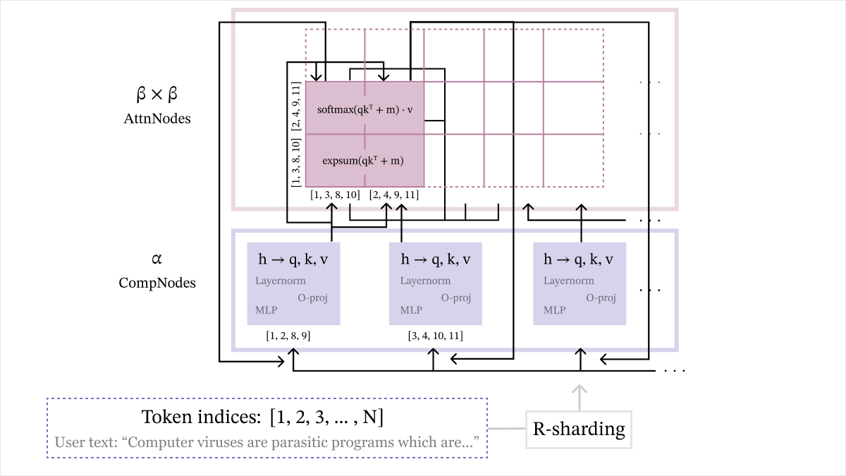
High-level representation of Cascade.
Do We Defend Against Our Attack?
In the beginning of the series, we mentioned our goal was an obfuscation scheme that defends against the vocab-matching attack, whilst retaining the exact results of normal inference. To make this notion well-defined, we need to explicitly adapt vocab-matching to the token-sharded setting. The attack we outlined in the previous blog post assumes that the adversary has access to the full hidden state matrix, so it does not work out-of-the-box for token-sharded hidden states.
Generalizing Our Attack to Token-Sharding
Suppose an adversary does not have access to all rows of hidden states , but only of them, say , with in strictly increasing order.
Our modification to our original attack again utilizes the autoregressive property to reduce the search space. This proceeds iteratively, where we initialize and .
- Assume at this point that we have deciphered tokens . We iterate through all possible combinations of tokens and perform forward passes, until we find a hidden state matrix whose -th row matches the observed . This takes at most forward passes.
- We set tokens to the ones that gave a match in Step 1. Then, we increment , repeat Step 1 if , and terminate if .
Note that this attack only allows recovery of tokens up to and including the last hidden state index , but not for tokens .
Below is an example of this generalized attack when the adversary has access to , meaning . First, a search over candidate first tokens that matches against allows recovery of in at most forward passes. Once is known, a search over candidate second and third tokens with matching to can recover in at most forward passes. Next, with known, matching against lets us recover . Finally, matching to recovers . Recovery of is not possible with this attack — although these tokens could be inferred from the previous tokens through other means, e.g. with punctuation.
 Demonstration of generalized attack for token-sharded hidden states. Colors represent different iterations of the procedure, with the maximum forward pass cost highlighted underneath.
Since we placed no restrictions on the choice of , it seems at first glance that this attack works on any token-sharded hidden state matrix, and can decipher the full input sequence if . This would appear to immediately render Cascade insecure, as the CompNode with the last hidden state row could obtain the full input sequence.
What’s the catch here? The attack cost.
In our attack, we see that at the th iteration, we could require up to passes in the worst case. For a typical LLM, the vocabulary size is on the order of hundreds of thousands. In Gemma-2-2B-IT, with , a gap of entails forward passes. Here, even if each forward pass took one nanosecond, the worst-case runtime would be nearly 30 billion years, more than double the current age of the universe!
In other words, this attack is infeasible when gaps are large enough.
What does “large enough” mean here? This is not clear-cut, as it can depend on the use case, adversarial computational power, and many other security parameters. So, to formalize our security analysis, we introduce the vocab-matching threshold , which is the maximum value of where forward passes can be performed by the adversary. In context of the attack, this means that once a gap is at least , the attack times out at the th iteration. This is the key condition that ensures Cascade is secure to vocab-matching.
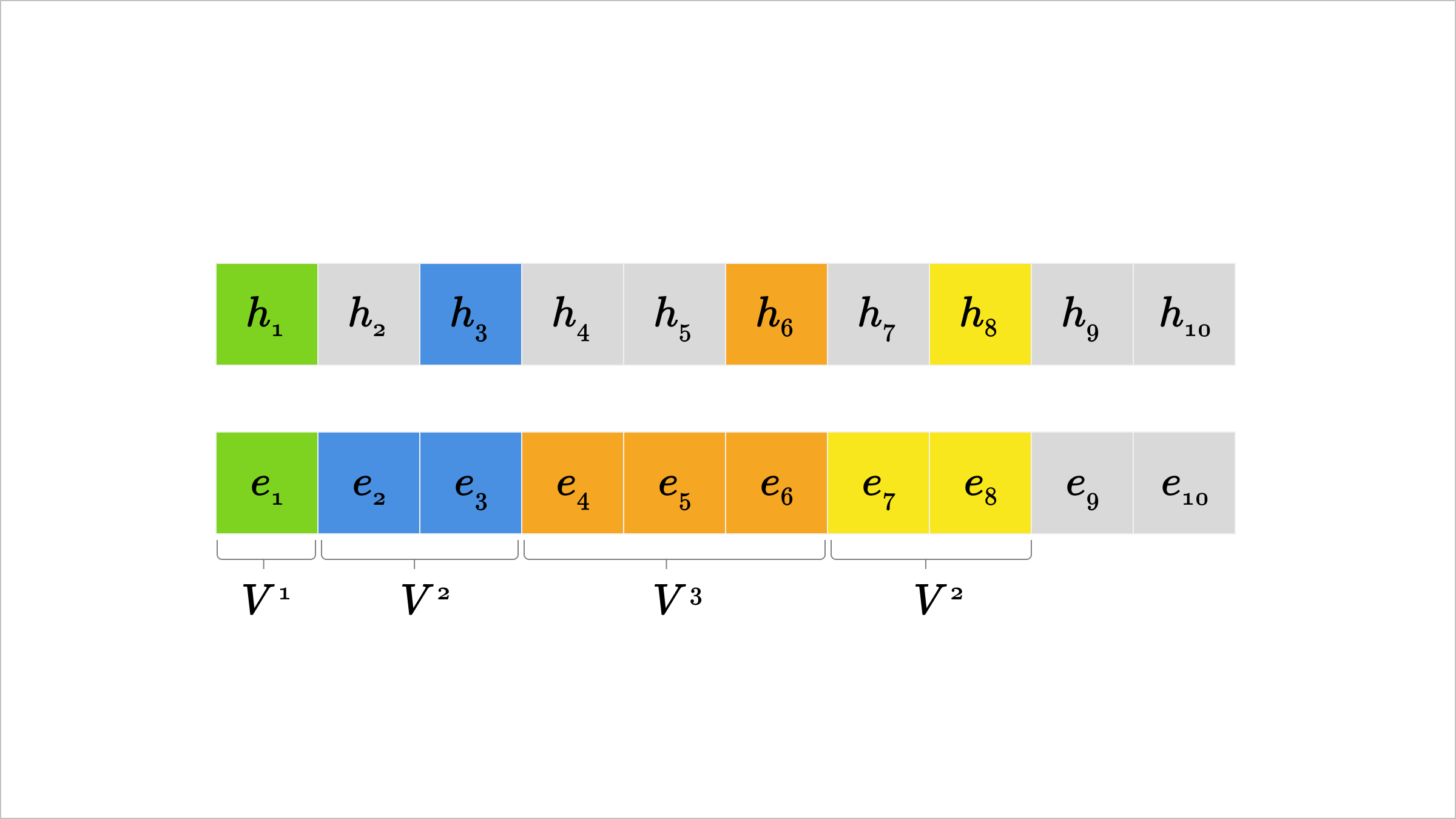
-Sharding
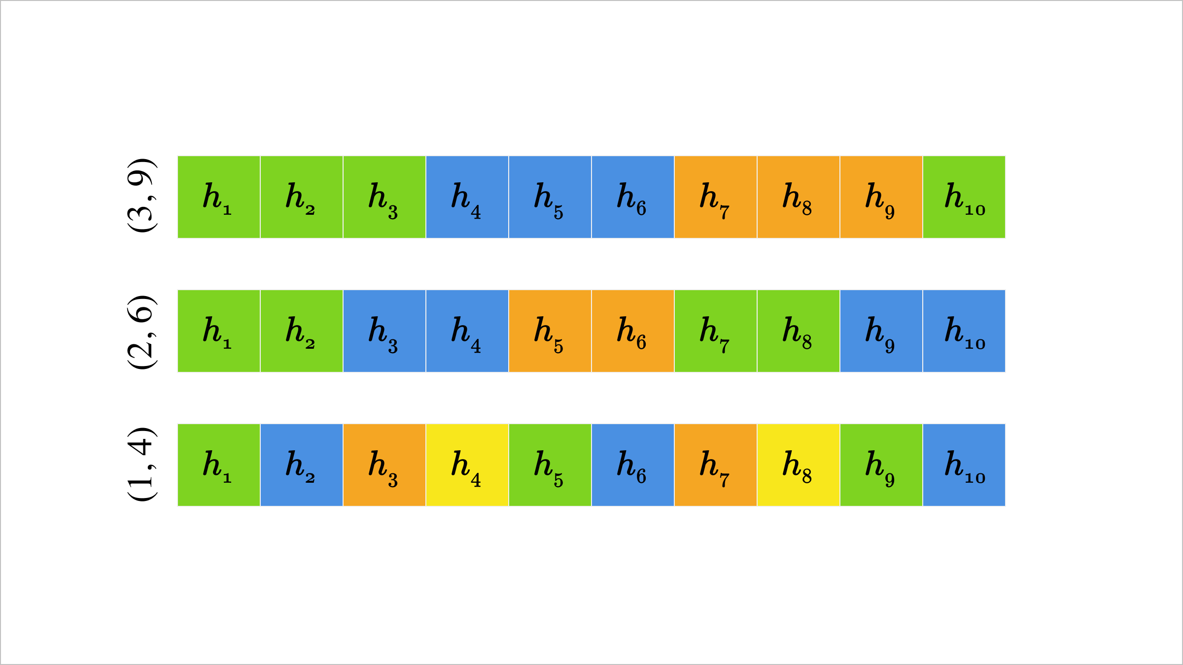
Although we have generalized our attack to arbitrary choices of token (row) indices , it will be useful to focus on a particular sharding setup called -sharding. Formally, this is a form of R-sharding where each consists of clusters of consecutive elements separated by . For instance, below, we highlight , , and sharding schemes when . The case has in green, in blue, and in orange.
Visual representation of -sharding, where boxes of the same color represent a single shard .
The motivation for this kind of sharding is that we uniformly spread gaps. This will simplify our analysis on gap sizes, although many other similar schemes could be considered.
Large Gaps Ensure CompNode Security
We can now explain why, when only considering leakage from R-shards of hidden states to CompNodes, -sharding with a large enough gap size is secure to vocab-matching.
For simplicity, consider the first CompNode, which has hidden state rows at some layer with indices . They already know tokens from Layer 0 token embeddings, so the next gap in their search is , and this requires on the order of forward passes. Recalling the vocab-matching threshold, this means is likely to make the attack infeasible.
A concrete example is shown below, for the -sharding setup and the first (green) CompNode. While the CompNode can recover in work without issue, the next gap of size to requires up to forward passes. If the vocab-matching threshold was set to , we would consider this infeasible.
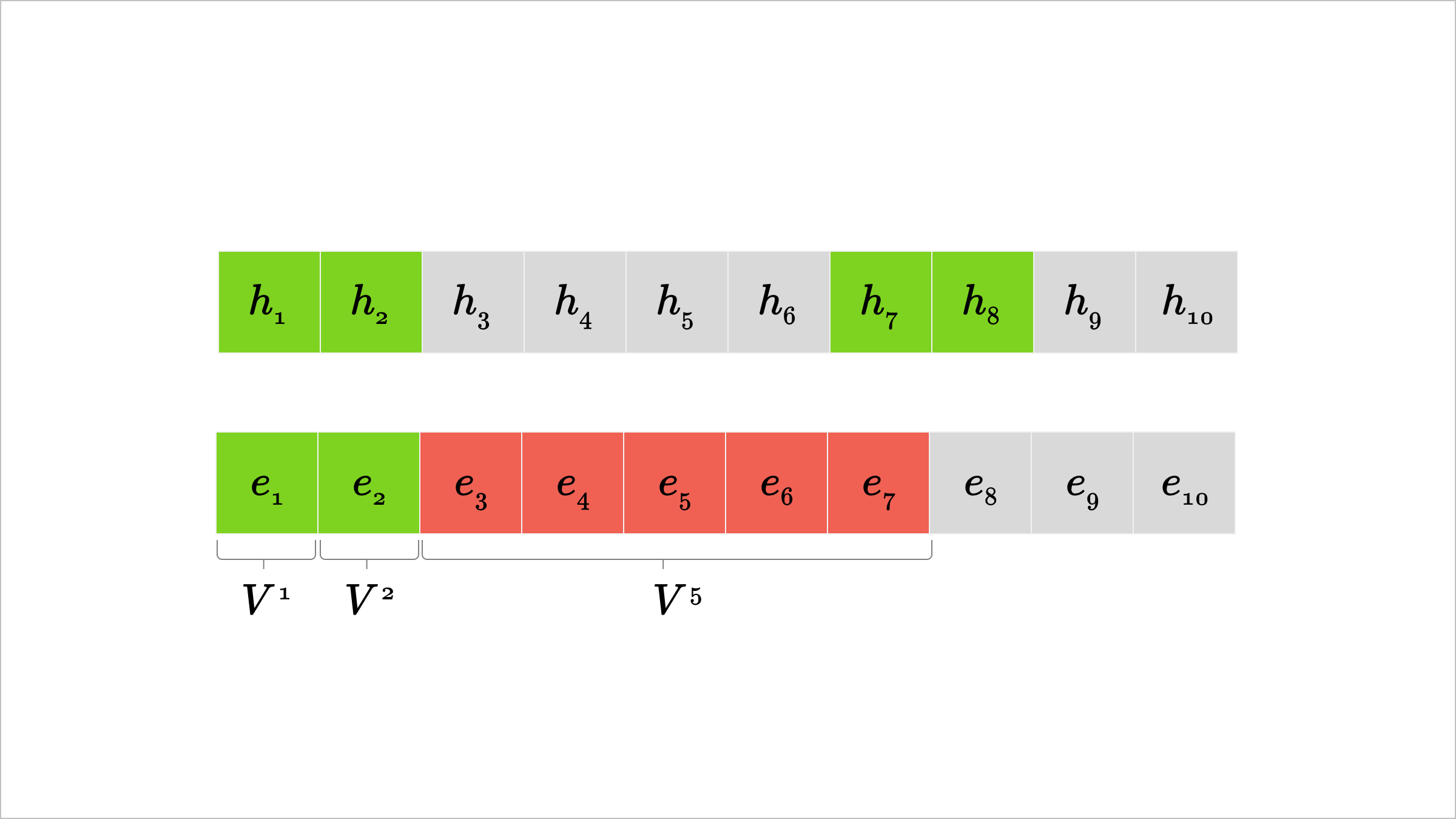
Visual representation of attack failure for large token gaps in -sharding.
We finally note that this is not a comprehensive security analysis, since there are other important shards leaked to CompNodes (e.g. max and expsum shards, and partial attention outputs), which could potentially reveal different information than R-sharded hidden states. Still, it turns out that these additional shards do not allow vocab-matching if the gap size is again sufficiently large. For further details, see our paper.
-Splitting Improves AttnNode Security
Now that we have explained when vocab-matching is infeasible for CompNodes, we turn to AttnNodes. In our scheme, AttnNode receives all query rows with indices in and all key rows with indices in . At first glance, assuming the shards were chosen to ensure CompNode security, one might expect AttnNodes to be secure. However, this is not the case: AttnNode gets access to query and key rows spanning indices , which has double the number of indices that any CompNode accesses if !
Concretely, we consider potential security risks at Layer , where the query, key, and value rows are linear projections of (normalized) token embeddings, and thus could reveal the same amount of information as their corresponding embeddings. Essentially, CompNode has access to tokens in and AttnNode has access to tokens in .
How do we prevent AttnNodes from getting this many tokens in the prompt? We consider an approach which makes sharding at the AttnNode level more granular than R-sharding. Formally, we alternatingly split each into subsets, to form a new partition of tokens with . Now, AttnNode receives query rows in and key rows in , so their token (row) access has been decreased by a factor of . This approach is called -splitting.
While our motivation for -splitting came from reducing direct token access, the question still remains: does this prevent vocab-matching? The answer is affirmative, in the same way as our analysis of CompNodes. If is large enough, there are still large enough gaps between consecutive clusters in , so as long as a gap is , the attack times out.
What Do Learning-Based Attacks Reveal?
While we have enumerated security considerations from our attack, a comprehensive analysis must consider other forms of reversal on hidden states. Most existing attacks in the literature are learning-based, which we break into the cases of Layer 0 (textual) and later layers.
Layer 0
At Layer 0, CompNodes individually receive some tokens in the prompt. While we would expect little security risk from revelation of a few scattered tokens, there are serious issues when gaps between the tokens are not too large, due to the risk of token infilling. To test this, we use ModernBERT-large to estimate the prior distribution on input tokens and thus infill tokens. Below, we see ROUGE scores for reconstructed tokens are quite low for larger (cluster size) and (CompNode count), with scores below for indicating nearly random reconstruction and good security.
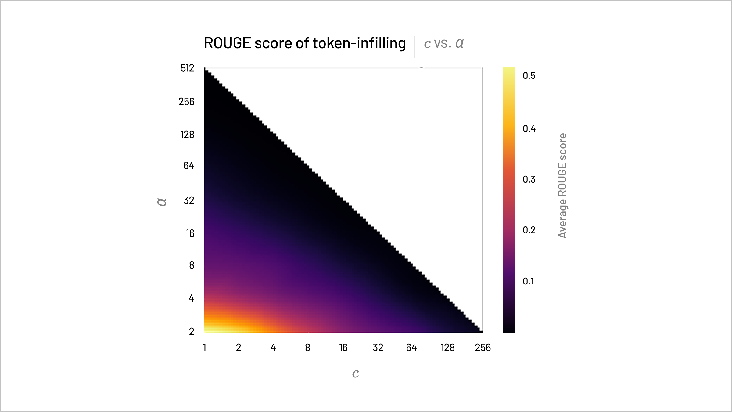
ROUGE-L scores for Layer 0 token infilling in Gemma-2-2B-IT with ModernBERT-Large tend to decrease as , the cluster size, and , the CompNode count, increase.
The analysis for AttnNodes is similar. Indeed, we remarked earlier that at Layer 0, AttnNode essentially has access to tokens with indices in , so they essentially have the same information as a CompNode with shard . Thus, for sufficiently large , we ensure AttnNodes cannot perform vocab-matching, by referencing CompNode security.
Later Layers
To assess the capability of learning-based attacks that aim to infill at later layers, we follow the approaches of Wan et al and Morris et. al. We fine-tune Gemma-2-2B-IT on -masked inputs to CompNodes at Layer 1, with a bidirectional mask to match the infilling task, and then evaluate on Layer 1 representations. As we see below, the resulting ROUGE evaluation scores decrease as and increase; and achieves a score near or below, indicating little reconstruction success by the learning-based attack.
| 0.701 | 0.467 | 0.349 | |
| 0.427 | 0.290 | 0.230 | |
| 0.355 | 0.222 | 0.191 |
ROUGE-L scores for Layer 1 infilling in Gemma-2-2B-IT tend to decrease as , the cluster size, and , the CompNode count, increase.
For AttnNodes, the use of -splitting gets ROUGE scores near those of CompNodes for . Following the same approach as above for , but now using -split -masked inputs to AttnNodes at Layer 1 for various values of , we see below that achieves comparable reconstructibility to CompNodes.
| ROUGE-L | |
|---|---|
| 2 | 0.3057 |
| 3 | 0.2643 |
| 4 | 0.2376 |
ROUGE-L scores for Layer 1 infilling in Gemma-2-2B-IT, using -splitting, tend to decrease as increases, with achieving comparable performance to the CompNode score.
Thus, measures like -sharding and -splitting protect Cascade against existing learning-based attacks, for particular choices of those security parameters.
Cascade vs. SMPC: Scalability vs. Security
We have shown that Cascade with a large-gap -sharding setup defends well against learning-based attacks, as well as our generalized vocab-matching attack. However, we emphasize that Cascade does not make any claims about provable security, as cryptographic schemes like SMPC do. We can only offer statistical security, like in our demonstrated low ROUGE-L scores of existing attacks on hidden state shards.
Given the gap in security strength between Cascade and SMPC, why should we choose Cascade? The main benefits are practical deployment and scalability, as SMPC schemes are often infeasible for larger models. For instance, one recent state-of-the-art SMPC scheme, Puma, takes around minutes for a full forward pass from Llama-2-7B on a 128-token prompt. This is far too slow to be used in any real-time inference service.
We compare Cascade runtimes for various values of to existing SMPC schemes MPCFormer and Puma on Bert-Base and Bert-Large:
| Scheme | Bert-Base (s) | Bert-Large (s) |
|---|---|---|
| MPCFormer | 55.32 | 141.22 |
| Puma | 33.91 | 73.72 |
| Cascadeα=1 | 0.32 [0.31, 0.36] | 1.01 [0.97, 1.09] |
| Cascadeα=4 | 0.59 [0.51, 0.69] | 1.57 [1.44, 1.73] |
| Cascadeα=8 | 0.74 [0.62, 0.96] | 1.58 [1.27, 1.97] |
| Vanilla | 0.09 [0.08, 0.12] | 0.27 [0.20, 0.99] |
Total runtime means and 95% confidence intervals in seconds over 100 trials, for a single 128-token prompt forward pass on Bert-Base and Bert-Large for MPCFormer, Puma, and various settings of newmethod. Higher α corresponds to increased node counts and security.
We run the above across machines on a WAN; for Cascade , we use 6 machines, and for , we use 18 machines. We see that Cascade is up to 100x faster than MPCFormer and Puma. We also note the sublinear growth in runtime as increases, so that scaling to large numbers of nodes (which offers the most security) does not significantly compromise runtime.
We also measure communicated bytes for each of the methods; these are shown in the table below. Cascade requires several orders of magnitude fewer communicated bytes than existing SMPC methods, supporting operation even in poor bandwidth network conditions.
| Scheme | Bert-Base (GB) | Bert-Large (GB) |
|---|---|---|
| MPCFormer | 12.089 | 32.577 |
| Puma | 10.773 | 27.246 |
| Cascadeα=1 | 0.009 | 0.025 |
| Cascadeα=4 | 0.038 | 0.101 |
| Cascadeα=8 | 0.076 | 0.203 |
Total gigabytes (GB) communicated for a single forward pass on Bert-Base and Bert-Large for MPCFormer, Puma, and newmethod with various settings. A prompt length of 128 is used.
Finally, we show the scalability of Cascade to larger model sizes below:
| Model Name | Model Size (Parameters) | Mean Runtime (s) |
|---|---|---|
| Bert-Base | 110M | 0.70 |
| Bert-Large | 335M | 1.33 |
| Llama-3.2-1B-Instruct | 1B | 2.67 |
| Llama-2-7B | 7B | 12.71 |
| Llama-2-13B | 13B | 22.72 |
Cascade with and no -splits scales well to larger models, Runtimes here are averages over 100 trials for a 128-token prompt.
Cascade further scales well to larger models like Llama-2-13B, and generally seems to sublinearly increase in runtime with model size. This is because for all per-token operations in transformer blocks, there is no computational overhead in Cascade’s sharding setup relative to vanilla inference. All overhead comes from attention, but it is ultimately negligible compared to the heavy matrix multiplication costs present in vanilla inference.
Thus, even as Cascade is not cryptographically secure, due to its efficiency and scalability, it holds immediate promise as a viable protocol for private large-scale LLM inference.
Summary
Our work on Cascade stems from the following fundamental question: How much information about input tokens do partial LLM hidden states leak? We motivated this inquiry from our work on the vocab-matching attack in the previous blog post, which showed full hidden states, even when shuffled, leak the full input sequence. Our results show that by choosing a sharding scheme which places sufficient gaps between tokens, the resulting sharded hidden states reveal little to no information about the input, from the perspective of both vocab-matching and existing attacks in literature. As Cascade reveals such sharded states to nodes in isolation, this provides strong statistical evidence for its security. While Cascade cannot offer the same strict privacy guarantees as SMPC schemes, it is a highly efficient protocol that offers potential for faster private LLM inference on larger hosted models.
To cite this blog post, please use:
@misc{cascade-token-sharded-inference,
  title={Cascade: Token-Sharded Private LLM Inference},
  author={Rahul Thomas, Louai Zahran, Erica Choi, Micah Goldblum, Arka Pal},
  year={2025},
  howpublished=\\url{ritual.net/blog/cascade}
}Disclaimer: This post is for general information purposes only. It does not constitute investment advice or a recommendation, offer or solicitation to buy or sell any investment and should not be used in the evaluation of the merits of making any investment decision. It should not be relied upon for accounting, legal or tax advice or investment recommendations. The information in this post should not be construed as a promise or guarantee in connection with the release or development of any future products, services or digital assets. This post reflects the current opinions of the authors and is not made on behalf of Ritual or its affiliates and does not necessarily reflect the opinions of Ritual, its affiliates or individuals associated with Ritual. All information in this post is provided without any representation or warranty of any kind. The opinions reflected herein are subject to change without being updated.